A Data Analytics using R Topic

What is PCA?

PCA for Dimensionality Reduction

Large datasets have many columns and variables. Having many variables (called features) makes the data high dimensional. Imagine a dataset with 100 features. To represent the data points on a graph, we would need 100 axes, one for each feature.

Principal Component Analysis (or PCA) is one method of identifying the most important axes with the most variance. Transforming your data to the new axes, called Principal Components, allows you to see the data from an improved perspective. Plotting data using the Principal Components instead of the original features can make clusters and patterns more apparent. Not only this, PCA is a simple way to discard the less important features to reduce the dimensionality.

Problems at High Dimensions

Say you wanted to train a statistical learning algorithm to distinguish between groups or classes in the data. For this learner to perform well it needs a large sample set. Feeding the algorithm with a representative training sample will make a learner better at predicting classes. Gathering these examples in high dimensional space poses problems. This is because high dimensional spaces are very big and more space has to be searched.

There are more problems than just gathering examples. As the number of dimensions increases, the Euclidean distance between points increases. Consequently, the data becomes more sparse and dissimilar making it more difficult for our learner to group points together by class.

The issue attributed to high dimensional datasets for machine learning algorithms is known as the Curse of Dimensionality.

Principal Component Analysis (or PCA) can help. Lets’s take a look at how.

How to do PCA in R

I generated simulated data with 30 observations for each of the three classes. Each observation has 100 different variables. To make the different classes distinct in some way, each class cluster has a different mean. Let’s visualise a snapshot in just two dimensions with the first two columns.

# obs is the data with 100 variables
plot(obs, col = c(rep("black",30), rep("blue", 30), rep("red", 30)), pch=19)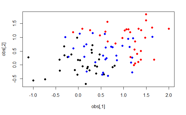

You can see there are three colours representing the three different classes. However, the groups overlap quite a bit. Let’s apply PCA to make the clusters more apparent. To do this we use the prcomp function in R. Let’s plot the first and second Principal Components now.

pr.out <- prcomp(obs)

plot(obs, col = c(rep("black",30), rep("blue", 30), rep("red", 30)), pch=19)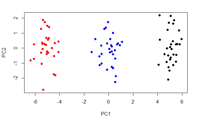

The three classes become much more apparent. This is an improved visualisation of the data. The training process of a clustering algorithm like K-means will benefit from PCA.

You can see that the classes are spread along PC1. We can plot the proportion of the total variance that each PC accounts for.

pr.sd <- pr.out$sdev # standard deviations


pr.var <- pr.sd ^ 2 # variance

pve <- pr.var/sum(pr.var) # proportion of variance explained

plot(pve[1:20],
     xlab = 'Principal Component',
     ylab = 'PVE',
     type = 'b',
     col = 'blue')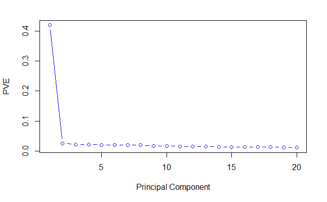

Principal Component one always has the greatest proportion of variance explained (PVE) followed by PC2 and PC3 etc. In my data, 40% of the variance is along PC1 alone. The PVE decreases from then on. We can see that the PC1 axis is the most important because the data is separated most along it. Therefore, PC1 will be the most valuable variable for a classifier to consider.

So for this dataset, how much can we reduce the dimensionality by? Let’s plot the cumulative proportion of variance explained against the number of PCs considered with cumsum.

cumsum(pve)

plot(cumsum(pve),
     xlab = 'PC',
     ylab = 'CPVE',
     type = 'b',
     col = 'red')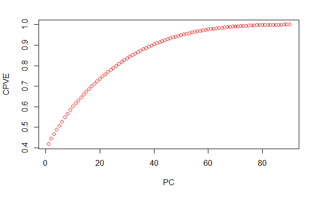

With just 50 PCs, we can half the dimensionalilty of the dataset while retaining over 90% of the variance of the data. Our classifier algorithm can learn to distinguish classes much more effieciently with less dimensions.

In summary then, PCA can reduce the dimensions of the dataset while keeping the most important infromation in the data.