Quick start: Reinforcement Racer

Reinforcement learning is the often forgotten sibling of supervised and unsupervised machine learning. But now, with its important role in generative AI learning, I wanted to touch on the subject with a fun introductory example. Fun projects like these can always teach you a lot.

I was inspired by YouTuber Nick Renotte (video: https://www.youtube.com/watch?v=Mut_u40Sqz4) and retried his Project 2 from the two-year-old tutorial. In this tutorial, we teach a model to race a car.

F1 drivers learn from experience, and so does a reinforcement learning agent. Let’s look at teaching such an agent to race through training and making it learn from repeated experience.

A quick recap of Reinforcement Learning (RL)

The docs of RL library, called “Stable Baselines3”, states the following,

“Reinforcement Learning differs from other machine learning methods in several ways. The data used to train the agent is collected through interactions with the environment by the agent itself (compared to supervised learning where you have a fixed dataset for instance).”

https://stable-baselines3.readthedocs.io/en/master/guide/rl_tips.html

So in RL, there is the concept of an agent/model interacting with its surroundings and learning through rewards. Actions that lead to achieving the goal are rewarded and so are reinforced as being “good” actions.

For the environment, i.e. our race track, we can use the already created, “CarRacing” environment from the “Gymnasium” project – the actively developed fork of OpenAI’s project called “Gym”. Gymnasium helps to get started quickly with reinforcement learning with many pre-made environments.

CarRacing environment. The agent controls a car.

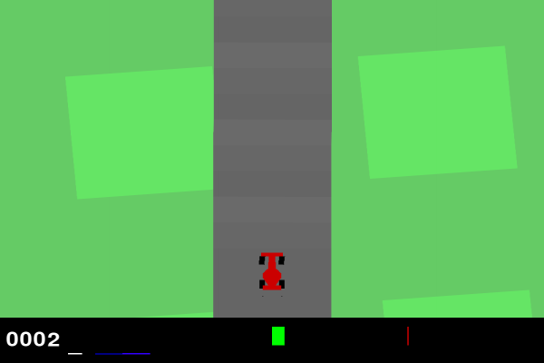
In CarRacing, the reward is negative (-0.1) for every frame and positive (+1000/N) for every track tile visited, where N is the total number of tiles visited in the track. Hence, the car is encouraged to move as quickly as possible and visit new parts of the track. The negative reward penalises staying still as the agent is encouraged to get to the finish asap. The positive reward encourages the car to visit new parts of the track as quickly as possible.

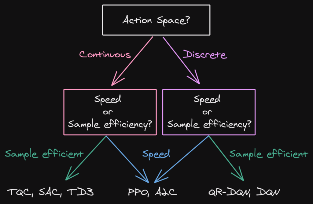
For our agent, I will use the PPO algorithm from the Stable Baselines3 library which comes with a general but good choice of hyperparameters for its models.

PPO: Proximal Policy Optimization

PPO is an algorithm for training RL agents. It has been used before in the fine-tuning of large language models via Reinforcement learning from human feedback (RLHF: https://en.wikipedia.org/wiki/Reinforcement_learning_from_human_feedback).

In PPO, the agent selects random actions which get less random over time as it learns. PPO is conservative in its learning process and makes sure not to change its policy (essentially its brain) by changing too much in each update. Constraining updates in this way leads to consistent performance, stability and speedy learning. However, this may also cause the policy to get stuck in a sub-optimal method for success. PPO seems to work well for this task in a short amount of time without requiring huge memory resources. It’s great to get started.

Read more about it: https://spinningup.openai.com/en/latest/algorithms/ppo.html

Stable baselines3 guide to choosing agents https://stable-baselines3.readthedocs.io/en/master/guide/rl_tips.html.

Whereas Nick used the stable baslines3 library directly, I will use Stable Baseline’s “RL zoo” – a framework for using Stable Baselines3 in an arguably quicker and more efficient way – all on the command line. RL Zoo docs: https://stable-baselines3.readthedocs.io/en/master/guide/rl_zoo.html

Training with RL Zoo – Reinforcement boogaloo

I found an easy way to get training our PPO agent (see: https://github.com/DLR-RM/rl-baselines3-zoo). I followed the installation from source (this requires git). I also recommend you create a virtual environment for all the dependencies.

git clone https://github.com/DLR-RM/rl-baselines3-zoo

Your system is probably different from mine and my commands for the command line are aimed at Linux/MacOS so you may need to translate some commands for your system.

Really make sure to have all the dependencies!

pip install -r requirements.txt
pip install -e .

Now let’s start training. Specify the algorithm (PPO), the environment (CarRacing-v2) and the number of time-steps (try different numbers!). For example you can try 500000 time steps.

python -m rl_zoo3.train --algo ppo --env CarRacing-v2 --n-timesteps 500000

This may take a few minutes. If you’re on Linux and get error: legacy-install-failure you may also need to install a few more packages.

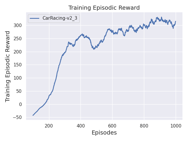
sudo dnf install python3-devel<br>sudo dnf install swig<br>sudo dnf groupinstall "Development Tools"

Once training is complete, you can visualise the learning process by plotting the reward over time/training episodes.

python scripts/plot_train.py -a ppo -e CarRacing-v2 -y reward -f logs/ -x steps

Increasing rewards with episodes indicates that the agent is learning.

Record a video of your latest agent with

python -m rl_zoo3.record_video --algo ppo --env CarRacing-v2 -n 1000 --folder logs/

I tested the agent after 4,000,000 time steps of training (~2hr for me) and got this episode below – what a good run!

RL zoo allows you to continue training if you want to improve it.

python train.py --algo ppo --env CarRacing-v2 -i logs/ppo/CarRacing-v2_1/CarRacing-v2.zip -n 50000

Thanks for reading!

/e/OS: An Easy and Private Custom ROM

My Samsung S9 is usable hardware. However, the Android version feels slow and is no longer supported by Samsung – i.e., it hasn’t received security updates since 2022. One option is to sell it and buy a new phone. Another option is to install a new operating system on it! Thereby reducing e-waste and saving money.

I can install a new OS for free on my S9, improving the phone’s longevity and giving it a fresh new look. Let me introduce /e/OS (“e OS”).

/e/OS is a modified version of Android, a custom ROM, that is maintained independently of Samsung or Google’s Android. /e/OS is also a fork of an operating system called LineageOS and removes almost all of the closed-source Google code from Android.

/e/OS is open-source Android at its core, with no Google apps or Google services accessing your personal data. So if privacy is important to you, /e/OS is a good option.

There are other custom ROMs out there but I find /e/OS to work well with most apps. It also looks clean and is easy to install with their Easy Installer app which walks you nicely through the process.

Is Privacy Traded for Functionality?

For most applications, /e/OS is great, but not all. The App Lounge is your Play Store/App Store but focuses on Privacy. I like how it scores an app’s privacy out of 10. I try to minimise the number of low privacy-scoring apps on my phone.

The App Lounge has pretty much all apps that you would want. I can get working Instagram and Discord – even if they are not the most privacy-respecting applications. However, it was hard to find Discord and some common apps were not readily findable. The App Lounge is also filled with some weird and random apps too but at least it doesn’t have ads all over like Google Play Store.

I find for messaging, most apps work fine except Facebook Messenger which didn’t work for me. One surprisingly great app is NewPipe, a client for YouTube. NewPipe gives you all the perks of YouTube Premium for free and doesn’t even track you as YouTube does. The consequence is that you are not provided with recommended content.

So /e/OS has me covered for YouTube and messaging. Navigation/maps, however, is a big trade-off (in my opinion).

The default maps app is Magic Earth. Magic Earth’s routing can be quite off, especially for the London Underground. It will recommend poor routes – I don’t really trust it. Google Maps is far superior as a service. I use TFL Go in tandem with Magic Earth when navigating London.

As for e-mail, I can use my Gmail account just fine, as well as my Murena e-mail that I got with my Murena cloud account (Murena is behind /e/OS). More on that later.

/e/OS has some advanced privacy features which I like. You can toggle on the use of the Tor network, and you can block Trackers on apps.

When using /e/OS, there is a small trade-off between functionality and privacy, but not in all aspects.

/e/OS – e Foundation

Murena Cloud

Your /e/OS phone has good (optional) integration with Murena Cloud. Part of the point of /e/OS is moving away from Google. Murena Cloud is an alternative to Google Cloud but with only 1GB free compared to Google’s 15GB of free space.

However, I like Murena’s transparency in telling me which country my data is being held. They also give you an e-mail alias if you don’t want to always give out your e-mail.

Closing

/e/OS looks good and works well for me (apart from Maps). /e/OS is not for everyone and I think it depends on the person – the advanced privacy features are probably not worth the small functionality trade-off for most people.

An S9 specific issue: I couldn’t find a way to map the Bixby button to anything. I would also like to have a cap on battery charging (cap at 85%) like my S21 has to prevent overcharging and increase battery longevity. Clearing all open tabs was also not obvious to me and should be more prominent. Another problem was enabling 2FA for Murena cloud but I managed it – this needs to be easier.

/e/OS has good privacy out of the box and most Meta and Google apps like Instagram, WhatsApp and Gmail still work – it’s good they’re there in case you still really need them. However, it almost defeats the point of the OS.

Overall a great OS and alternative to Google and Apple operating systems.

Self-hosting with Mini PCs: Discord bot & Minecraft server

Not a data science blog today! I wanted to briefly share some project ideas for self-hosting and just say that Mini PCs are great! Mini PCs can be powerful and quiet little desktops, but, they can also function as servers.

I got my hands on two Intel NUCs, which are small form-factor computers. It’s just like a normal desktop but can fit in your hands (~10 x10 cm).

If you leave them with networking and no I/O, they will sip power (~30 Watts) and act like a little server.

NUCs and other similar mini PCs such as the Antec Asrock have many use cases. For example, host websites (like this one!), be home media servers (with Jellyfin or Plex software) and be used for Home Automation servers (and more).

Below are two examples: Hosting a Discord bot and Bedrock Minecraft Server. As for software prerequisites, my NUC has Ubuntu server, Python, Docker and Docker Compose already installed.

Discord bot

Let’s create our own Discord bot and self-host it. First, you want to want to visit https://discord.com/developers, create an application and add a bot. You will need to copy the token and save it somewhere safe. For permissions, it depends on the bot, but usually I enable send and read messages at the least. For Privileged Gateway Intents, I would usually enable all.

A typical bot could start like this

import discord
intents = discord.Intents.all()
intents.members = True

This gives your bot the ability to receive member-related events. Next, we could make our bot invoke commands when a user types in ‘$’ in chat:

from discord.ext import commands
client = commands.Bot(command_prefix = "$", intents = intents)

@client.event
async def on_ready():
print('We have logged in as {0.user}'.format(client))

The on_ready() function will let us know when the bot is connected to Discord and ready to start processing events.

If we want the bot to say hello when we type $hello in the discord server we can use “context” (ctx).

@client.command()
async def hello(ctx):
    await ctx.send('Hello!')

Don’t forget to run the bot with your token client.run("TOKEN"). You can add your bot to your server using the OAuth2 URL generator in the Developer Portal, ticking send and read messages, and pasting the URL into the browser

I recommend using ctx for sending messages – it can make things easier. The context contains information about the message that triggered the command. This includes the channel, server, and author of the message.

You can run the bot with python3 name_of_bot.py in the terminal.

Check out my GitHub for a Discord bot that uses the Natural Language Toolkit (NLTK) Python package to find the most negative user (silly usage I know!). Fabio-RibeiroB/NLPdisrespectBOT: Discord Bot for Sentiment Analysis (github.com)

This is not a dedicated server for my bot so let’s containerise the application and let it run in the background.

I don’t want my secret token in the container in case I want to share the image so I created a .env file with TOKEN=my_token (ignore quotes) and add this to a .gitignore and .dockerignore files. In the bot script, you will then need to load the env variables using the python-dotenv library.

Our Dockerfile could look like this:

FROM python:3
WORKDIR /app
COPY . .
RUN pip install -r requirements.txt
CMD ["python", "sentimental_analysis_bot.py"]

This assumes you have a requirements.txt file with all your dependencies.

While in the directory of the bot, let’s build the image from a Dockerfile and name it.

docker build -t my_container_name -f Dockerfile .

Now we run the image as a container and pass it to the .env file and run it in the background

docker run -d --env-file=.env my_container_name

After entering the container I can see that there is no .env file. Great!

Minecraft Bedrock server

No need to spend $5/month on a server when you can host it yourself. Thanks to the itzg/minecraft-bedrock-server – Docker Image | Docker Hub docker image, having your own Minecraft server is not too difficult. I have only played around with the Bedrock version but I believe the Java steps are similar.

You will need docker to pull the image above (see the GitHub or Docker hub page for more info) and I recommend using docker-compose to get the container up in the background (command: docker-compose up -d).

As for configurable settings, I would enable the “allow list” which specifies which players can join the server; it’s just a security feature. However, the easiest way to add people to the allow list from the terminal is not clear to me. In the end, I just entered the running container (command: sudo docker exec -it my_server_name bash) and edit the allow list JSON by installing vim (apt update && apt upgrade && apt install vim). Here is an example allowlist.json.

[{"ignoresPlayerLimit":false,"name":"Your_name","xuid":"Your_xuid"}]

To find your xuid use this site: https://www.cxkes.me/xbox/xuid.

Once the container is running, you must set up port forwarding – WikiHow has a nice guide for doing this.

Below is an example docker-compose.yml that uses itzg’s Minecraft image, and set’s the Minecraft server to be survival mode, online, have an allow_list and set the name. If you ever want to change anything you can edit this file or server.properties and restart the container. For example, you may want to allow cheats.

version: '3.4'

services:
  bds:
    image: itzg/minecraft-bedrock-server
    restart: always
    environment:
      EULA: "TRUE"
      GAMEMODE: survival
      DIFFICULTY: easy
      ONLINE_MODE: "true"
      ALLOW_LIST: "true"
      SERVER_NAME: "My World"

    ports:
      - 19132:19132/udp
    volumes:
      - bds:/data
    stdin_open: true
    tty: true

volumes:
  bds: {}

To join the server, make sure you are on the allow list, type the server IP (same public IP as the NUC) and the port in “add server” on Minecraft.

I haven’t found a better way yet to change the allow list other than installing vim on the container and editing the allow_list.json file. Or you can just disable the allow list so any can join if you are having trouble with friends connecting.

Class Balancing: SMOTE & Variations

Frequency and Bias

An important consideration in any classification task is class frequency. Class imbalances are problematic because the classifier becomes less sensitive to the minority classes. Consider a training set with a majority class A and minority B. An algorithm trained on this imbalanced data will develop a bias toward predicting A just because it appears more often. Another dataset could in theory contain more of B, for example. This classifier would function poorly in this case because it learned a preference for A.

To avoid this bias, perform class balancing. There are different ways to accomplish balancing. One method is to oversample the minority classes by duplicating observations. However, oversampling can cause the algorithm to overfit, and the data becomes skewed toward the replicated observations. Alternatively, one could undersample the majority class, leading to a loss of valuable information for a classifier [1]. I prefer to maintain as much information as possible.

In this article, I explain variations of oversampling, including using existing observations from the minority to synthesise new data. Balancing via artificial means is known as Synthetic Minority Oversampling Technique, or SMOTE [3].

SMOTE and Tomek Links

A data point can be represented as a vector, where each entry of the vector is an attribute. SMOTE works by first selecting a feature vector from the minority class at random. Then, the algorithm chooses a random neighbouring feature vector from k-nearest (usually five) neighbours. The new, synthesised, feature vector lies at an arbitrary point along the line connecting the two [3]. Fig.1 depicts synthetic data generation in SMOTE with an example dataset.

Fig.1: How SMOTE generates new points by connecting feature vectors. Image from imblearn [2].

The problem with SMOTE is that it can generate noise by interpolating points between outliers [2], and alone does not necessarily improve on the more straightforward random oversampling method. It is unlikely that SMOTE adds any additional information by using existing data, but SMOTE still shifts the bias toward the minority class [2]. Applying SMOTE may increase the sensitivity of the minority class but could decrease accuracy and precision. The authors of SMOTE found that combining SMOTE with under-sampling methods can improve classification performance [3].

To address some issues with SMOTE, particularly the case of synthetic noise, there is a modified version, SMOTE+Tomek, which tries to clean the feature space of synthetic noise. SMOTE+Tomek removes a majority class point with the nearest neighbour of another class. The pair of two closeby opposing types is called a Tomek link and is illustrated in Fig.2 [2].

Fig.2: Illustration of a Tomek link [2].

Undersampling the majority class with Tomek links thus removes boundary cases between classes and class label noise.

Another variation of SMOTE is SMOTE+ENN. Considered an improvement to removing Tomek links, SMOTE+ENN deletes the k-nearest neighbours as well as the points of the Tomek link [4]. There are more variations of SMOTE, including KMeans+SMOTE [5] which applies KMeans clustering before SMOTE.

It is important to note that class balancing is performed after the train-test split otherwise SMOTE will interpolate points between test data in training data. In this scenario, the new feature vectors in the training set could leak information about the location of points in the test data.

An alternative method to deal with imbalanced data and avoid SMOTE entirely is using balanced ensemble classifiers. In balanced ensemble methods, bootstrapping can be used to sample the data so that the constituent classifiers (e.g., trees in a forest) train on subsets with the classes present in equal amounts [6].

Example in Python: imblearn library

from imblearn.pipeline import make_pipeline
from sklearn.ensemble import RandomForestClassifier
from imblearn.over_sampling import SMOTE

pipeline = [SMOTE(random_state=0),
           RandomForestClassifier(random_state=0, min_samples_split=4, n_estimators=500)
          ]
model = make_pipeline(*pipeline)
model.fit(X_train, y_train)
y_pred = model.predict(X_test)

See more on the imblearn website: https://imbalanced-learn.org/dev/references/generated/imblearn.over_sampling.SMOTE.html#

References:

[1] Ma Y, He H. Imbalanced learning: foundations, algorithms, and applications. John
Wiley & Sons; 2013

[2] imblearn library documentation; By the Imbalanced-learn developers. Available from:
https://imbalanced-learn.org/dev/index.html.
[3] Chawla NV, Bowyer KW, Hall LO, Kegelmeyer WP. SMOTE: synthetic minority over-
sampling technique. Journal of artificial intelligence research. 2002;16:321-57.
[4] Batista GE, Bazzan AL, Monard MC, et al. Balancing Training Data for Automated
Annotation of Keywords: a Case Study. In: WOB; 2003. p. 10-8.
[5] Last F, Douzas G, Bacao F. Oversampling for imbalanced learning based on k-means
and smote. arXiv preprint arXiv:171100837. 2017.
[6] Chen C, Liaw A, Breiman L, et al. Using random forest to learn imbalanced data. University of California, Berkeley. 2004;110(1-12):24.
d case studies. MIT Press; 2020.

ML App with Flask

You built an ML with TensorFlow or Sci-kit learn and now want it deployed on a website. This article is a quick guide on loading an ML model in Python and using it to make predictions on a web app with Flask. This is based on my image classifier app found on my GitHub Fabio-RibeiroB/image_classifier_app: App to classify happy or sad images (github.com). In this app, the user uploads a file and presses predict. Specifically, the user uploads images for binary classification. It all depends on your model. You can change this code to upload CSV data instead, for example.

I appreciate this article is high-level and lacking detail. It is more than an outline to make it as short-form as possible. To see more, check out my aforementioned repo on GitHub. Anyway, let’s begin.

Save and Load

Let’s say you have a Sequential model that you compiled.

model = Sequential()
....some model
....
model.compile(....)

Now save the model, for example, as a .h5 file. I saved mine in a “models” folder. You can also use pickle to dump and load models as .pkl files.

from tensorflow.keras.models import load_model
import os
model.save(os.path.join('models','model.h5'))

Now load it in your Flask app.

from flask import Flask, render_template, request, redirect, flash, session # useful flask modules
from werkzeug.utils import secure_filename # security
import logging

logging.basicConfig(level=logging.DEBUG)
logging.info('program starting')

from tensorflow.keras.models import load_model
model = load_model('models/model.h5') # loaded model

Static Uploads Folder

We also need a folder where we can upload data for the model. Make a directory called static, and within that, a directory called uploads.

UPLOAD_FOLDER = './static/uploads'
ALLOWED_EXTENSIONS = {'png', 'jgp', 'jpeg'} # change depending on model
app = Flask(__name__)
app.secret_key = b'somesecretkey'
app.config['UPLOAD_FOLDER'] = UPLOAD_FOLDER

def allowed_file(filename):
    """
    Check the uploaded data is correct format
    """"
    return '.' in filename and \
          filename.rsplit('.', 1)[1].lower() in ALLOWED_EXTENSIONS

Routes and Prediction

Now I create the necessary routes in your app that makes a prediction. We will later make a home.html will allow us to start a prediction. The predict.html page shows the results.

@app.route('/')
def home():
    return render_template('home.html')

@app.route('/predict', methods=['POST'])
def predict():
    file = request.files('file')
    # check uploaded file is okay in upload folder
    if file and allowed_file(file.filename):
        filename = secure_filename(file.filename)
        data_path = os.path.join(app.config['UPLOAD_FOLDER'], filename)
   
        file. save(data_path) # save data
        # read data in for example with pandas
        prediction = model.predict(data) # in my example prediction is one number, a probability.

        # remember to delete file after use

        os.remove(data_path)
        return render_template('predict.html', data=prediction)
   
if __name__ == "__main__":
    app.run(debug=True)

The above code saves the valid data in the uploads folder and loads the data. For example, you could load your data into a pandas data frame. The /predict route passes the prediction variable containing a single prediction. The prediction variable is passed to predict.html to render the result on the web page. If your model outputs a lot of predictions, like a CSV of predictions, these lines will need to be modified. You probably want the user to download the predictions as a CSV instead of displaying the results on the screen. In this case, you need a download button in your HTML.

However, continuing my example, we have a home page called home.html with a form for the user to upload data. I simply removed the rest of my HTML tags to declutter the code snippet below. See my repo for the entire HTML file.

In home.html

<form method="POST" action="{{url_for('home')}}"   enctype=multipart/form-data>
    <input type=file name=file>
    <input type=submit value=predict>
</form>

And now for prediction.html. This page will simply output the results with a back button.

{{data}}
<form>
<input type="button" value="Try again" on    click="history.back()">
</form>

Flask run, and the app should be running in local host.

SQLite in Python

Getting started

SQLite is a common SQL database engine. In this blog, I will go over how you can connect and query a SQLite database in Python.

Let’s import the necessary libraries for this example, and establish a connection to a database. We will be using the sqlite3 library and pandas.

import sqlite3
import pandas as pd
conn = sqlite3.connect('supermarket.db') # connect to a supermarket database

To execute SQL commands, we need to create a cursor object. Let’s use the cursor to create a table called shops which will contain basic information about our supermarket stores (shop ID, size, postcode) . The store sizes are small, medium and large.

cursor = conn.cursor() # create a cursor
cursor.execute("CREATE TABLE shops(shopid VARCHAR(100) PRIMARY KEY, Store_size VARCHAR(30), Postcode VARCHAR(8))")

So, cursor.execute() executes SQL commands.

We can insert data into the table using the INSERT command. If we do this, use conn.commit() to save the data to the table.

However, in this example, we have a pandas DataFrame called shops_df that we wish to insert into our SQL table called shops. It has the same columns as our shops table. If you’re more familiar with pandas than SQL like me, I will use pandas to clean data first. Only after this will I want to store the data in an SQL database.

The to_sql() function allows us to write records in a DataFrame to an SQL database.

shops_df.to_sql('shops', conn, if_exists='append', index=False) # write shops_df to shops table

Queries

The cursor behaves like an iterator object. We can use a for loop to retrieve all rows from a SELECT statement. To make it easier to query in future, I’ll create a query function.

def query(q):
    try:
        for row in cursor.execute(q):
            print(row)
    except Exception as e:
        print("Something went wrong... ", e)

query('SELECT * FROM shops')

We can also save the results of a query by assigning it to a variable. The variable will be a list of tuples. A tuple for each row.

q="SELECT shopid, Postcode FROM shops"
query_results = cursor.execute(q).fetchall() # save results as a list of tuples

Storing results from a query like this can allow you to represent table data with graphs. For example, if you had a table called sales in your database which has the shop profits, you could plot trends in sales. I will illustrate this now.

Above: A preview of the sales table which is in our SQLite database already

Let’s query the minimum, mean and maximum yearly sales…

c="""
SELECT shops.Store_size, sales.Year, MIN(sales.Sales), AVG(sales.Sales), MAX(sales.Sales)
FROM shops
JOIN sales
  ON shops.shopid = sales.shopid
GROUP BY shops.Store_size, sales.Year 
"""
query(c)
result = cursor.execute(c).fetchall()
Above: the results from our query

…next I plot the mean sales for medium sized stores against the year…

years=[] # store the year
means = [] # store the mean sales
size = 'medium'
for results in result:
    if results[0] == size:
        means.append(results[3])
        years.append(results[1])

plt.plot(years, means, linestyle = 'dashed', marker = 'o', ms= '5')
plt.title(f"{size} store mean sales")
plt.xlabel("year")
plt.ylabel("sales")
plt.savefig(f"{size}_store_mean_sales.png")
plt.show()
Above: the mean sales for stores that are medium sized

Now we are done, close the connection to the database.

conn.close() # don't forget to close the connection afterwards

I hope this blog was helpful for getting started with the sqlite3 library, to connect to a database, and use a cursor to execute SQL commands in python.

PCA in R

A Data Analytics using R Topic

What is PCA?

PCA for Dimensionality Reduction

Large datasets have many columns and variables. Having many variables (called features) makes the data high dimensional. Imagine a dataset with 100 features. To represent the data points on a graph, we would need 100 axes, one for each feature.

Principal Component Analysis (or PCA) is one method of identifying the most important axes with the most variance. Transforming your data to the new axes, called Principal Components, allows you to see the data from an improved perspective. Plotting data using the Principal Components instead of the original features can make clusters and patterns more apparent. Not only this, PCA is a simple way to discard the less important features to reduce the dimensionality.

Problems at High Dimensions

Say you wanted to train a statistical learning algorithm to distinguish between groups or classes in the data. For this learner to perform well it needs a large sample set. Feeding the algorithm with a representative training sample will make a learner better at predicting classes. Gathering these examples in high dimensional space poses problems. This is because high dimensional spaces are very big and more space has to be searched.

There are more problems than just gathering examples. As the number of dimensions increases, the Euclidean distance between points increases. Consequently, the data becomes more sparse and dissimilar making it more difficult for our learner to group points together by class.

The issue attributed to high dimensional datasets for machine learning algorithms is known as the Curse of Dimensionality.

Principal Component Analysis (or PCA) can help. Lets’s take a look at how.

How to do PCA in R

I generated simulated data with 30 observations for each of the three classes. Each observation has 100 different variables. To make the different classes distinct in some way, each class cluster has a different mean. Let’s visualise a snapshot in just two dimensions with the first two columns.

# obs is the data with 100 variables
plot(obs, col = c(rep("black",30), rep("blue", 30), rep("red", 30)), pch=19)

You can see there are three colours representing the three different classes. However, the groups overlap quite a bit. Let’s apply PCA to make the clusters more apparent. To do this we use the prcomp function in R. Let’s plot the first and second Principal Components now.

pr.out <- prcomp(obs)

plot(obs, col = c(rep("black",30), rep("blue", 30), rep("red", 30)), pch=19)
The data plotted using Principal Components (PC) 1 and 2

The three classes become much more apparent. This is an improved visualisation of the data. The training process of a clustering algorithm like K-means will benefit from PCA.

You can see that the classes are spread along PC1. We can plot the proportion of the total variance that each PC accounts for.

pr.sd <- pr.out$sdev # standard deviations


pr.var <- pr.sd ^ 2 # variance

pve <- pr.var/sum(pr.var) # proportion of variance explained

plot(pve[1:20],
     xlab = 'Principal Component',
     ylab = 'PVE',
     type = 'b',
     col = 'blue')
The data varies along PC1 much more than any other component

Principal Component one always has the greatest proportion of variance explained (PVE) followed by PC2 and PC3 etc. In my data, 40% of the variance is along PC1 alone. The PVE decreases from then on. We can see that the PC1 axis is the most important because the data is separated most along it. Therefore, PC1 will be the most valuable variable for a classifier to consider.

So for this dataset, how much can we reduce the dimensionality by? Let’s plot the cumulative proportion of variance explained against the number of PCs considered with cumsum.

cumsum(pve)

plot(cumsum(pve),
     xlab = 'PC',
     ylab = 'CPVE',
     type = 'b',
     col = 'red')
Cumulative Proportion of Variance Explained with the number of Principal Components

With just 50 PCs, we can half the dimensionalilty of the dataset while retaining over 90% of the variance of the data. Our classifier algorithm can learn to distinguish classes much more effieciently with less dimensions.

In summary then, PCA can reduce the dimensions of the dataset while keeping the most important infromation in the data.